Welcome to TourCalc’s documentation!

Contents:

• Introduction & Used Algorithms
  • Creation of input data
  • Longest Processing Time algorithm – Approximate solution
    • Splitting of disciplines with dynamic creation of competition areas
    • Partially used competition areas
    • Discipline Change - penalty factor for changing a discipline
  • Free parameters
    • Order of the disciplines
    • Happiness value
    • Discipline Change - penalty factor for changing a discipline
  • The best results
  • Glossary
• Installation and Usage
  • Use deployed app
  • Installation own instance
• Tutorial
  • Read in tournaments
    • Read in example tournament
    • Read in tournament - from file
  • Create a new tournament
    • Final block
    • Type of break
  • Adding of participants
    • Adding “random” participants
  • Save the input
  • Change settings per day
  • Understand the results
  • Known Problems & improvements
    • GUI is not visible
    • Other issues
• tourcalc
  • tourcalc package
    • cal_cat()
    • calculate_fight_time()
    • descition_matrix()
    • distr_cat_alg()
    • getdata()
    • heatmap()
    • minloadtatami()
    • plot_schedule_time()
    • read_in_file()
    • write_tour_file()
    • Submodules
• Credits
  • Author
  • Contributors

Introduction & Used Algorithms

Scheduling of sports tournaments can be approximated with the so-called multiprocessor scheduling, a known NP-hard computer science problem. With this, the goal is to find a minimum end-time \(ET_{min}\) of the tournament by distributing of the different categories on a given number of competition area s \(T\). A category here is defined in agreement with the Organization and Sporting Code (Version 3.1) OSC of the Ju-Jitsu International Federation (JJIF) under paragraph 1.3 (Disciplines, Divisions and Categories). However, the program shall also provide a base for integrating more disciplines or other sports.

Creation of input data

The first step is the creation of the input data. Since the names of categories in the tournament calculator are based on 1.3.3 of the OSC, the user only needs to select one or more age division [1] and discipline [2]. All categories are created, and the user is asked to add the number of athletes/couples for each category. Based on the competition systems (as defined in the OSC under 4.4) the number of matches \(N_{m}(n_{a})\) for each category is known and can be described the following.

\[\begin{split}N_{m}(n_{a})= \begin{cases} d(n_{a}) , &n_{a} < 7\\ 2 \cdot n_a - 5, & n_{a} \geq 7 \\ \end{cases} \\ \text{ with } d(n_{a} \to N_{m}; 0 \to 0, 1 \to 0, 2 \to 3, 3\to 3, 4 \to 6, 5 \to 10, 6 \to 9)\end{split}\]

Fig. 1 shows the number of matches \(N_{m}\) as a function of the number of athletes \(n_{a}\).

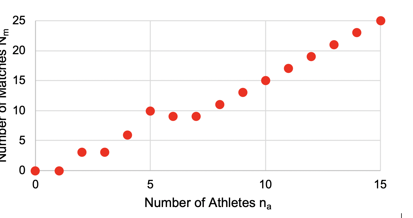
Fig. 20 Number of matches \(N_{m}\) as a function of the number of athletes \(n_{a}\).

The individual time \(l\) for each category can be calculated as on the number of matches \(N_{m}\) times the average match time per discipline \(<t_{x}>\) (See :ref:`avtime`_ average match time per discipline). The average match time covers the span between starting one match and starting of the next match, including interruptions of the fight and the change of the fighters. This value is based on the experience but also used in other competition software. It may vary based on the place and the tournament time and can be individually adjusted in the software source code.

Table 3 average match time per discipline

Discipline	Average match time \(<t_{x}>\)
	Adults	U21	U18	U16
Jiu-Jitsu	8 min	7 min	6 min	8 min
Fighting	7 min	7 min	7 min	6 min
Duo	7 min	7 min	7 min	5 min
Show	4 min	4 min	4 min	4 min

The individual time \(l_{xy}\) is calculated as the following:

\[l_{yx}= N_{m} (n_{a} ) <t_{x}>\]

In total, the input data can be described the following: There are \(X\) disciplines. Each discipline has \(Y\) individual categories with each category an individual time of \(l_{xy}\). With this is:

\[\begin{split}L_{X} = \sum_{y=1}^Y l_{xy} \text{ and } \\ L_{tot} = \sum_{x=A}^X L_{x} = \sum_{x=A}^X \sum_{y=1}^Yl_{xy} ,\end{split}\]

where \(L_{x}\) is the total discipline time, and \(L_{tot}\) is the total time for the full tournament. For a better understanding, see Fig. 2 Visualization of an example input data set.

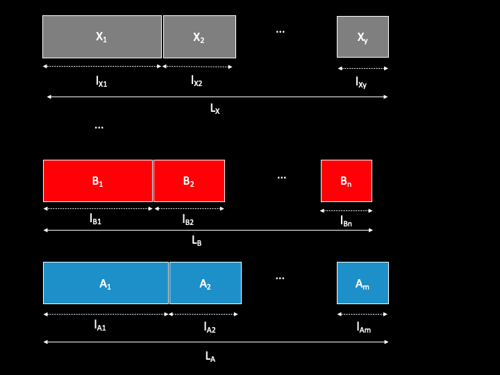
Fig. 21 Visualization of an example input data set. Here, the discipline \(A\) (in red) has \(M\) individual categories with each an individual duration of \(l_{AM}\). The total time of this discipline is \(L_A\)

Based on \(L_{tot}\) and the number of competition areas \(T\) an (artificial) perfect end-time \(ET_{perf}\) can be calculated the following:

\[ET_{perf}=\frac{L_{tot}}{T}\]

[1]

Adults, U21, U18 and U16 are supported in version 0.9.0

[2]

Jiu-Jitsu, Fighting, Duo and Show system are supported in version 0.9.0

Longest Processing Time algorithm – Approximate solution

The above-described problem can be approximately solved with the LPT algorithm (Longest Processing Time). It sorts the categories by their time \(l\), from longest to shortest. Then assigns them one after another to competition area \(T\) with the earliest end time so far. The logical assumption is made that only one category can be run per competition area at the same moment in time. Since the number of categories is usually minimal (<<1000), this straightforward algorithm seems to be a good starting point. However, it needs to be modified to fulfill the requirements of multi-discipline tournaments where not all referees can work on all competition areas due to individual qualifications.

In the JJIF, referees are specialized per discipline Referee. Therefore, it is crucial to minimize the change of disciplines for the individual competition areas \(T\) to avoid time-consuming commuting of qualified referees. To realize this, we choose to individually distribute the categories based on the above described LPT algorithm. This requires that for a given discipline, only needed competition areas are created. With this we used a so-called Euclidean Division: “Given two integers \(a\) and \(b\), with \(b \neq 0\), there exist unique integers \(q\) and \(r `such that :math:`a = bq + r\) and \(0 ≤ r < |b|\) where \(|b|\) denotes the absolute value of \(b\). In the above theorem, each of the four integers has its own name: \(a\) is called the dividend, \(b\) is called the divisor, \(q\) is called the quotient and \(r\) is called the remainder.”

In the case of the described data, we can define analogous a Euclidean Division with the following components:

1. dividend = total time of this discipline \(L_{a}\)

2. divisor = perfect end-time \(ET_{perf}\)

3. quotient = fully-used competition area \(N_{Ta}\)

4. remainder = remainder time` \(t_{r}\)

This converts the relation mentioned above to:

\[L_{a} = ET_{perf} \cdot N_{Ta} + t_{r} : a \in \{A, B, ⋯, X\}\]

where \(a\) is the name of the discipline. In our case, the dividend (total time of this discipline \(L_{a}\)) and the divisor (perfect end-time \(ET_{perf}\)) are known, and we want to compute the total number of tatamis.

The name fully competition areas used shall also imply that the end time of this competition area \(ET_{T}\) is as close as possible to perfect end-time \(ET_perf\). To calculate the number of fully-used competition areas per discipline for the above relation, one can use the well-known integer division in computer science:

\[N_{Ta}=INT \frac{L_{a}}{E_{perf}} : a \in ]\{A, B, ⋯, X\}\]

The remainder of the Euclidean Division is the remainder time \(t_r\) and might be used to create a new competition area it is called partially-used.

Since these mathematical expressions might not be familiar to many readers, we would like to give the following example:

Assuming we have a discipline A with a total discipline time of \(L_{A}\): 22:30 (=22 hrs and 30 min). The perfect end-time \(ET_{perf}\): of the tournament is 7:00 (7 hrs and 0 min).

The amount of fully used tatamis is

\[N_{Ta}=INT \frac{L_{a}}{E_{perf}} =INT \frac{22:30}{7:00} =INT(3.21)=3\]

The remainder time \(t_{r}\) is 1 hours and 30 minutes, which might need to be added either to the existing partially used competition area or created a new one.

If fully used or partially used, competition areas are created strongly depends on the total discipline time \(L_{x}\), the perfect end-time \(ET_{perf}\) and the amount of already created competition areas. We will discuss all distinct possibilities in dedicated examples below to make them better understandable.

In this first example, we want to explain the way the algorithm reacts when first called. We assume that \(L_{x}Lx < ET_{perf}\). The amount of fully used competition area is calculated in the first step, and those are created. Since \(L_{x}Lx < ET_{perf}\), the remainder time must be larger than zero. Since no other competition area exists, an additional partially-used competition area is created. This scenario is shown in Fig. 3.

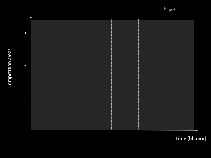
Fig. 22 Visualization of expected behavior with three identical competition areas, two disciplines and no placeholder time block

The LPT algorithm would tread all created competition areas the same, which would lead to an even distribution of end times \(ET_{T}\) for all three competition areas. However, is \(ET_{T}\) rather far away from the perfect end time, meaning we cannot consider these competition areas full used. If the next discipline is distributed, categories might be added to all the competition areas, introducing a change of the discipline that is not desired. To avoid this, we will add a placeholder time block at the partially used tatamis. The length of this placeholder time block is \(ET_{perf}-t_{r}\). It will be removed after the discipline allocation, leaving a very uneven distribution. This will allow the next discipline to be added on the partially-used competition area. This behavior is visualized in Fig. 4.

Fig. 23 Visualization of expected behavior with three identical competition areas, two disciplines and a placeholder time block

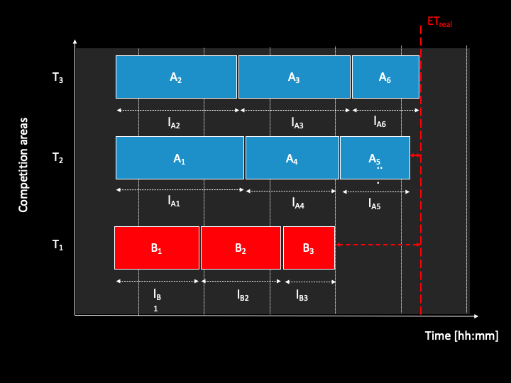
Changing the discipline will possibly need adjustment of the referees and the setup of the field of play. Therefore a penalty factor called discipline change is introduced. After the distribution of a discipline, this penalty factor is added. This parameter is \(T_{pen}\) and will be later varied. The animation in Fig. 5 shows the process.

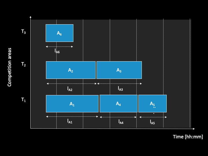
Fig. 24 Visualization of expected behavior with three identical competition areas, two disciplines and a placeholder time block and a penalty factor

Free parameters

The algorithm has three free and arbitrary parameters which need to be varied to find the optimal solution.

The answer of the algorithm depends on the order of the disciplines. Like shown in picture the following pictures the results will depend on the order of the disciplines.

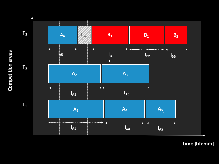
Fig. 25 Visualization of expected behavior with three identical competition areas, two disciplines, a placeholder time block, a penalty factor, starting with discipline A

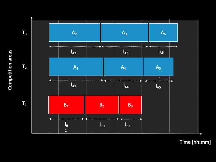
Fig. 26 Visualization of expected behavior with three identical competition areas, two disciplines, a placeholder time block, a penalty factor, starting with discipline B

Since there is no preferred order in general the algorithm will brute force try all of them which means it will use all possible permutations of the disciplines: Jiu-Jitsu, Fighting, Duo , Show. Since the number of disciplines is four in total 4! = 24 permutations are tested.

What makes an organizer “happy” is to end the tournament as short as possible and have all tatamis efficiently used. The second means to minimize the standard_deviation of the end times.

This can be computed as the minimum plus with the and a free parameter h.

\[ET_{min} + h * \sigma_{et}\]

The free parameter will run from 0, meaning the standard_deviation is not taken into account to 1 meaning that the standard_deviation is as equally important as the end time, in steps of 0.1.

The two pictures illustrate the parameter of the happiness value in two cases.

Like explained in previous chapters the change of a disciplines will result in a penalty. The default penalty time is 30 min. However the penalty time is rather arbitrary. Other results might be found by using different penalty factors. Therefore the parameter is varied from 15 min to 45 min.

The best results

The algorithm will run for each combination of happiness value and penalty factor and determines which is the permutation that gives the best result. If less than four disciplines are used for a day the “first” appearing permutation is used.

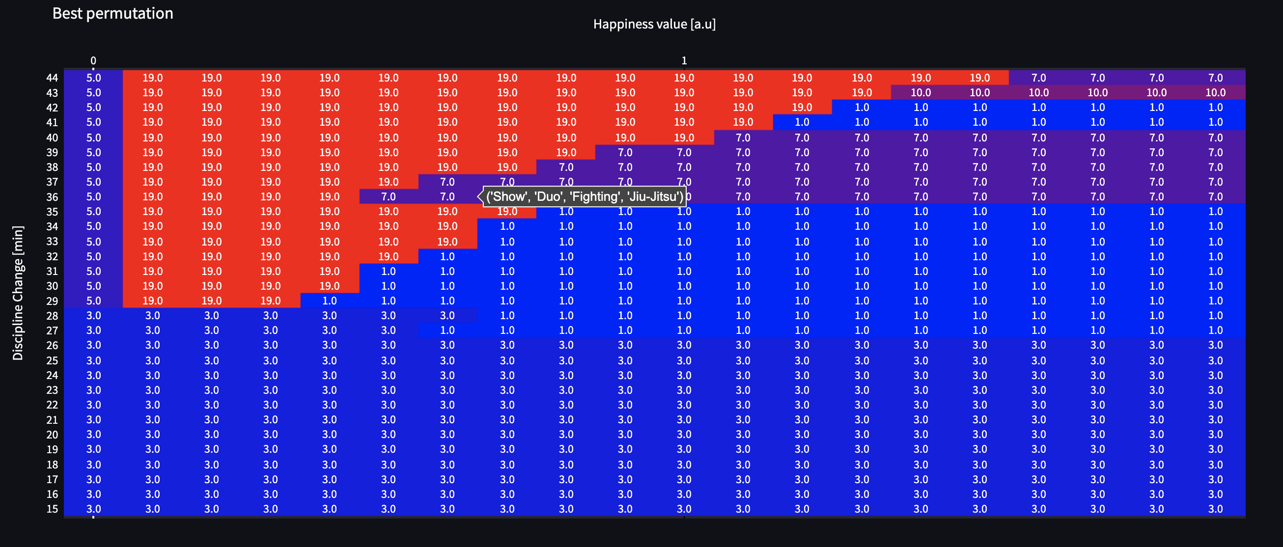
Fig. 27 Outcome of an event. For each combination of a happiness value and penalty factor the best permutation is found.

So what is now the best result for a tournament?

The answers will always be - it depends…

There might be restrictions on an event which the algorithms does not take into account.

In total, the algorithm will test:

1. 30 different penalty factors

2. 20 different happiness values

3. 24 permutations

And show you the best of those

\[30 \cdot 20 \cdot 24 = 14400\]

solutions.

Hopefully one will be the one that fits for your event.

Curious? You can test the algorithm on this webpage

Glossary

age division

An age division defines the minimum and maximum age of a participant

minimum end-time

The time after the last match has finished \(ET_{min}\)

discipline

Discipline is a branch of a sport that has a set of rules. For this program, disciplines might have a different time and different referees.

category

A category is a weight or gender division in a discipline.

competition area

A competition area can hold one match at the same time.

number of matches

The number of individual matches per category. It depends on the number of athletes/couples in this category.

athletes/couples

Participants in a category

individual time

The time for each category for all matches

average match time per discipline

This is the average time between the start if one match and the start of the next match

perfect end-time

Total fight time divided by the number of the competition area

fully-used

the fully used competition area

partially-used

partially-used competition area

placeholder time block

time block at partially used tatamis

Contributing

Everyone can contribute to TourCalc.

Indices and tables

• Index

• Module Index

• Search Page